RO simulations using `CRO` solver#

This tutorial illustrates how to use the pyCRO to solve the RO model.

[1]:

%config IPCompleter.greedy = True
%matplotlib inline
%config InlineBackend.figure_format='retina'

%load_ext autoreload
%autoreload 2

import warnings
warnings.filterwarnings("ignore")

import numpy as np
import matplotlib.pyplot as plt
import os
import sys
import calendar

sys.path.append(os.path.abspath("../../../"))

import pyCRO

RO Simulation Setup#

This is the simplest configuration for the RO model, using:

White noise: n_T = 1, n_h = 1.
Linear system: nonlinear terms (b_T, c_T, d_T, b_h) are zero. Note that All unspecified parameters default to zero.
Additive noise only: no multiplicative component (n_g = 2).

The RO equation is written as:

\(\displaystyle \frac{dT}{dt} = RT + F_{1}h + \sigma_{T}w_{T}\)
\(\displaystyle \frac{dh}{dt} = −\varepsilon{h} − F_{2}T + \sigma_{h}w_{h}\)

The following block sets parameters for the RO simulation.

[2]:

par = {'R': [-0.05],       # dT/dt=R*T (unit: month^-1)
       'F1': [0.02],       # dT/dt=F1*h (unit: K m^-1 month^-1)
       'F2': [0.9],        # dh/dt=-F2*T (unit: m K^-1 month^-1)
       'epsilon': [0.03],  # dh/dt=-epsilon*h (unit: month^-1)
       'b_T': [],          # dT/dt=(b_T)*(T^2) (unit: K^-1 month^-1)
       'c_T': [],          # dT/dt=-(c_T)*(T^3) (unit: K^-2 month^-1)
       'd_T': [],          # dT/dt=(d_T)*(T*h) (unit: m^-1 month^-1)
       'b_h': [],          # dh/dt=-(b_h)*(T^2) (unit: K^-2 m month^-1)
       'sigma_T': [0.2],   # dT/dt=(sigma_T)*(N_T) (unit: K month^-0.5 if n_T=1, K month^-1 if n_T=0)
       'sigma_h': [1.2],   # dh/dt=(sigma_h)*(N_h) (unit: m month^-0.5 if n_h=1, m month^-1 if n_h=0)
       'B': [],            # T/dt=(sigma_T)*(1+B*T)*(N_T) or dT/dt=(sigma_T)*(1+B*H(T)*T)*(N_T) (unit: K^-1)
       'm_T': [],          # d(xi_T)/dt=-m*T*(xi_T); (unit: month^-1)
       'm_h': [],          # d(xi_h)/dt=-m*h*(xi_h); (unit: month^-1)
       'n_T': [1],         # noise type for T (0: red noise, 1: white noise) (unitless)
       'n_h': [1],         # noise type for h (0: red noise, 1: white noise) (unitless)
       'n_g': [2]}         # multiplicative noise type for T (0: linear, 1: Heaviside linear, 2: omit this option)
                           # (note: only valid when B is not zero) (unitless)

The following block sets additional options for the RO simulation.

[3]:

IC = [1.0, 0.0]              # Initial conditions for T and h
N = 12 * 100                 # Simulation length in months (e.g., 100 years)
NE = 2                       # Number of ensemble members

The RO simulation can be run by setting four settings set above: par, IC, N, and NE.
The following block sets additional optional settings for the RO simulation.
The user may skip specifying these options. If the user doesn’t specify these options, the RO simulation runs with the default settings.

[4]:

NM = "EH"                    # Optional: Numerical integration method for
                             #           RO solver "EH" (Euler–Heun, default)
                             #           or "EM" (Euler–Maruyama)
dt = 0.1                     # Optional: Time step for numerical integration
                             #           in months. Default = 0.1
saveat = 1.0                 # Optional: Interval for saving outputs in months.
                             #           Default = 1.0
savemethod = "sampling"      # Optional: Output method. "sampling" saves
                             #           instantaneous values, "mean" saves
                             #           time-averaged values over each save
                             #           interval. Default = "sampling"
EF = None                    # Optional: External forcing dictionary.
                             #           If EF is None (or not specified),
                             #           it defaults to:
                             #           EF = {'E_T': [0.0], 'E_h': [0.0]}
                             #           Same format and interpretation as
                             #           other RO parameters. Example:
                             #           EF = {'E_T': [-0.01, 0.02, np.pi],
                             #                 'E_h': [-0.01]}
noise_custom = 999           # Optional: Noise specification.
                             #   - If None or not provided:
                             #     uses internally generated noise
                             #     (different each run; Default)
                             #   - If an integer: uses as the random seed for
                             #     reproducible noise with the reference number
                             #   - If ndarray: user-supplied noise
                             #     (shape must be (int(N/dt) - 1, 4))
                             #     The first two columns of the noise array are
                             #     applied to the main T and h equations.
                             #     The last two columns are used as noise terms
                             #     for the red noise processes.

[5]:

pyCRO.RO_solver?

Signature:
pyCRO.RO_solver(
    par,
    IC,
    N,
    NE,
    NM='EH',
    dt=0.1,
    saveat=1.0,
    savemethod='sampling',
    EF=None,
    noise_custom=None,
    verbose=True,
)
Docstring:
Numerical solution of the Recharge Oscillator (RO) model with stochastic forcing.

This function integrates the Recharge Oscillator (RO) system numerically using
either the Euler–Maruyama (EM) or Euler–Heun (EH) scheme. It includes
deterministic dynamics, stochastic noise (white or red), and optional
external forcing. Ensemble simulations are supported, with results returned
at user-specified output intervals.

Parameters
----------
par : dict
    Dictionary of model parameters with the following keys (as 1-element arrays):

    - ``'R'`` : float
        Damping parameter.
    - ``'F1'`` : float
        Feedback parameter relating thermocline depth to SST.
    - ``'epsilon'`` : float
        Thermocline damping parameter.
    - ``'F2'`` : float
        Feedback parameter relating SST to thermocline.
    - ``'sigma_T'`` : float
        Noise amplitude for SST.
    - ``'sigma_h'`` : float
        Noise amplitude for thermocline depth.
    - ``'B'`` : float
        Multiplicative noise coefficient (used when ``n_g`` = 0 or 1).
    - ``'n_T'`` : int
        Noise type in SST equation (``1`` = white noise, ``0`` = red noise).
    - ``'m_T'`` : array-like
        Memory kernel for red noise in SST equation (ignored if ``n_T=1``).
    - ``'n_h'`` : int
        Noise type in thermocline equation (``1`` = white noise, ``0`` = red noise).
    - ``'m_h'`` : array-like
        Memory kernel for red noise in thermocline equation (ignored if ``n_h=1``).
    - ``'n_g'`` : int
        Noise structure in SST equation:
        ``0`` = multiplicative, ``1`` = multiplicative + Heaviside, ``2`` = additive.
IC : tuple of float
    Initial condition ``(T0, h0)``:

    - ``T0`` : initial SST anomaly.
    - ``h0`` : initial thermocline depth anomaly.
N : float
    Total simulation length (time units).
NE : int
    Number of ensemble members.
NM : {'EM', 'EH'}, optional
    Numerical integration method. Default is ``'EH'`` (Euler–Heun).
dt : float, optional
    Numerical integration time step. Default is ``0.1``.
saveat : float, optional
    Output saving interval. Must be divisible by ``dt``. Default is ``1.0``.
savemethod : {'sampling', 'mean'}, optional
    Method for saving results:

    - ``'sampling'`` : store values every ``saveat`` steps (default).
    - ``'mean'`` : average values within each ``saveat`` interval.
EF : dict, optional
    External forcing with the following keys (as 1D arrays of length 5):

    - ``'E_T'`` : SST forcing coefficients.
    - ``'E_h'`` : Thermocline forcing coefficients.

    If ``None`` (default), no external forcing is applied.
noise_custom : {None, int, ndarray}, optional
    Specification of stochastic noise:

    - ``None`` (default): generate new Gaussian noise for each ensemble.
    - ``int`` : random seed for reproducible noise (same across ensembles).
    - ``ndarray`` of shape (NT-1, 4, NE) : user-provided noise realizations.
verbose : bool, optional
    If ``True`` (default), print detailed setup and progress messages.

Returns
-------
T_out : ndarray of shape (N_out, NE)
    SST anomalies from the numerical integration, after applying the saving scheme.
h_out : ndarray of shape (N_out, NE)
    Thermocline anomalies from the numerical integration, after applying the saving scheme.
noise_out : ndarray of shape (NT-1, 4, NE)
    Realizations of Gaussian noise used in the simulation.

Notes
-----
- White noise forcing corresponds to ``n_T = 1`` or ``n_h = 1``.
- Red noise forcing (``n_T = 0`` or ``n_h = 0``) requires a nonzero memory kernel ``m_T`` or ``m_h``.
- For the Euler–Maruyama method (``NM = 'EM'``) with multiplicative noise,
  an Ito-to-Stratonovich correction is applied automatically.

Examples
--------
>>> par = {
...     'R':[0.5], 'F1':[1.2], 'epsilon':[0.3], 'F2':[0.8],
...     'sigma_T':[0.2], 'sigma_h':[0.1], 'B':[0.05],
...     'n_T':[1], 'm_T':[0], 'n_h':[1], 'm_h':[0], 'n_g':[0]
... }
>>> IC = (0.1, -0.2)
>>> T, h, noise = RO_solver(par, IC, N=50, NE=5, dt=0.1, saveat=1.0)
>>> T.shape, h.shape
((51, 5), (51, 5))
File:      ~/codes/CRO/pyCRO/solver.py
Type:      function

RO Simulations#

Basic Usage#

``T_ro, h_ro, _ = pyCRO.RO_solver(par, IC, N, NE)``

This is the simplest setup:

T_ro and h_ro are arrays with shape (N, NE), where N is the number of time steps and NE is the number of ensemble members.
The third output (_) is the noise time series, with shape (N, 4, NE).

[6]:

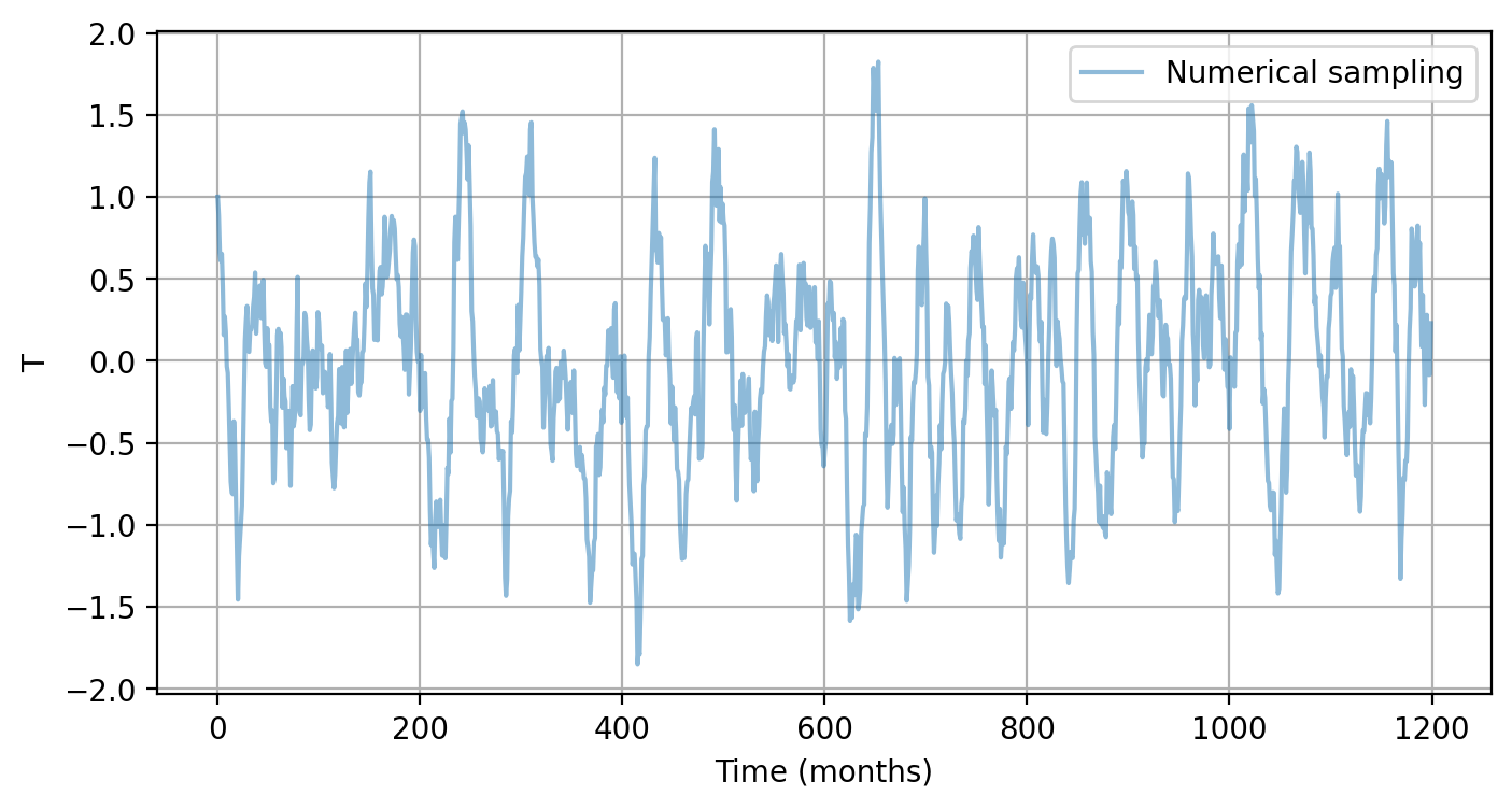
# Example 3-1. Solve RO with default settings
T_ro, h_ro, _ = pyCRO.RO_solver(par, IC, N, NE)

time_axis = np.arange(0, N, saveat)
num_en = 0 # plot first ensemble member solution of T

plt.figure(figsize=(8, 4))
plt.plot(time_axis, T_ro[:, num_en],  label='Numerical sampling',  alpha=0.5)
plt.xlabel("Time (months)")
plt.ylabel("T")
plt.legend()
plt.grid()
plt.show()

---------------------------------------------------------------------------------
Welcome to the CRO Solver! Your simulation setup is as follows:
---------------------------------------------------------------------------------
 - Total simulation length: N = 1200 months
 - Number of ensemble members: NE = 2
 - Numerical integration time step: dt = 0.1 months (default: 0.1)
 - Data output interval: saveat = 1.0 months (default: 1.0)
 - Initial conditions: IC = [T0, h0] = [1.0, 0.0]
 - Input parameters have the expected shapes.
 - 'n_T' = 1: White noise forcing in T; 'm_T' ignored.
 - 'n_h' = 1: White noise forcing in h; 'm_h' ignored.
 - 'n_g' = 2: Additive noise is used in the T equation; 'B' is ignored.
 - Numerical integration method: NM = 'EH' (Euler–Heun method; default)
 - Data saving method: savemethod = sampling (default)
 - External forcing is not given, therefore using
   EF = {'E_T': [0.0, 0.0, 0.0, 0.0, 0.0], 'E_h': [0.0, 0.0, 0.0, 0.0, 0.0]}.
 - noise_custom = None: System-generated noise is used and changes at every run.
---------------------------------------------------------------------------------
Numerical integration starting:
---------------------------------------------------------------------------------
---------------------------------------------------------------------------------
All steps successfully completed!
---------------------------------------------------------------------------------

Advanced Usage#

``T_ro, h_ro, _ = pyCRO.RO_solver(par, IC, N, NE, NM)``

``T_ro, h_ro, _ = pyCRO.RO_solver(par, IC, N, NE, NM, dt)``

``T_ro, h_ro, _ = pyCRO.RO_solver(par, IC, N, NE, NM, dt, saveat)``

``T_ro, h_ro, _ = pyCRO.RO_solver(par, IC, N, NE, NM, dt, saveat, savemethod)``

``T_ro, h_ro, _ = pyCRO.RO_solver(par, IC, N, NE, NM, dt, saveat, savemethod, EF)``

``T_ro, h_ro, _ = pyCRO.RO_solver(par, IC, N, NE, NM, dt, saveat, savemethod, EF, noise_custom)``

Optional arguments allow for more control.
Each additional argument gives more precise control over the solver.
Refer to the previous section for details on each argument.

[7]:

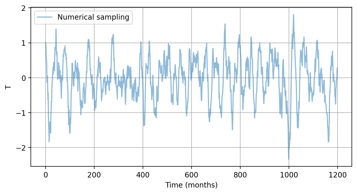
# Example 3-2. Solve RO with user-specified settings
T_ro, h_ro, _ = pyCRO.RO_solver(par, IC, N, NE, NM, dt, saveat, savemethod, EF, noise_custom)

time_axis = np.arange(0, N, saveat)
num_en = 0 # plot first ensemble member solution of T

plt.figure(figsize=(8, 4))
plt.plot(time_axis, T_ro[:, num_en],  label='Numerical sampling',  alpha=0.5)
plt.xlabel("Time (months)")
plt.ylabel("T")
plt.legend()
plt.grid()
plt.show()

---------------------------------------------------------------------------------
Welcome to the CRO Solver! Your simulation setup is as follows:
---------------------------------------------------------------------------------
 - Total simulation length: N = 1200 months
 - Number of ensemble members: NE = 2
 - Numerical integration time step: dt = 0.1 months (default: 0.1)
 - Data output interval: saveat = 1.0 months (default: 1.0)
 - Initial conditions: IC = [T0, h0] = [1.0, 0.0]
 - Input parameters have the expected shapes.
 - 'n_T' = 1: White noise forcing in T; 'm_T' ignored.
 - 'n_h' = 1: White noise forcing in h; 'm_h' ignored.
 - 'n_g' = 2: Additive noise is used in the T equation; 'B' is ignored.
 - Numerical integration method: NM = 'EH' (Euler–Heun method; default)
 - Data saving method: savemethod = sampling (default)
 - External forcing is not given, therefore using
   EF = {'E_T': [0.0, 0.0, 0.0, 0.0, 0.0], 'E_h': [0.0, 0.0, 0.0, 0.0, 0.0]}.
 - noise_custom = 999: seeded same noise.
---------------------------------------------------------------------------------
Numerical integration starting:
---------------------------------------------------------------------------------
---------------------------------------------------------------------------------
All steps successfully completed!
---------------------------------------------------------------------------------

Analytical Solutions of Linear RO With White Noise#

``T_ref, h_ref, _ = pyCRO.RO_analytic_solver(par, IC, N, NE)``

``T_ref, h_ref, _ = pyCRO.RO_analytic_solver(par, IC, N, NE, dt)``

``T_ref, h_ref, _ = pyCRO.RO_analytic_solver(par, IC, N, NE, dt, saveat)``

``T_ref, h_ref, _ = pyCRO.RO_analytic_solver(par, IC, N, NE, dt, saveat, savemethod)``

``T_ref, h_ref, _ = pyCRO.RO_analytic_solver(par, IC, N, NE, dt, saveat, savemethod, noise_custom)``

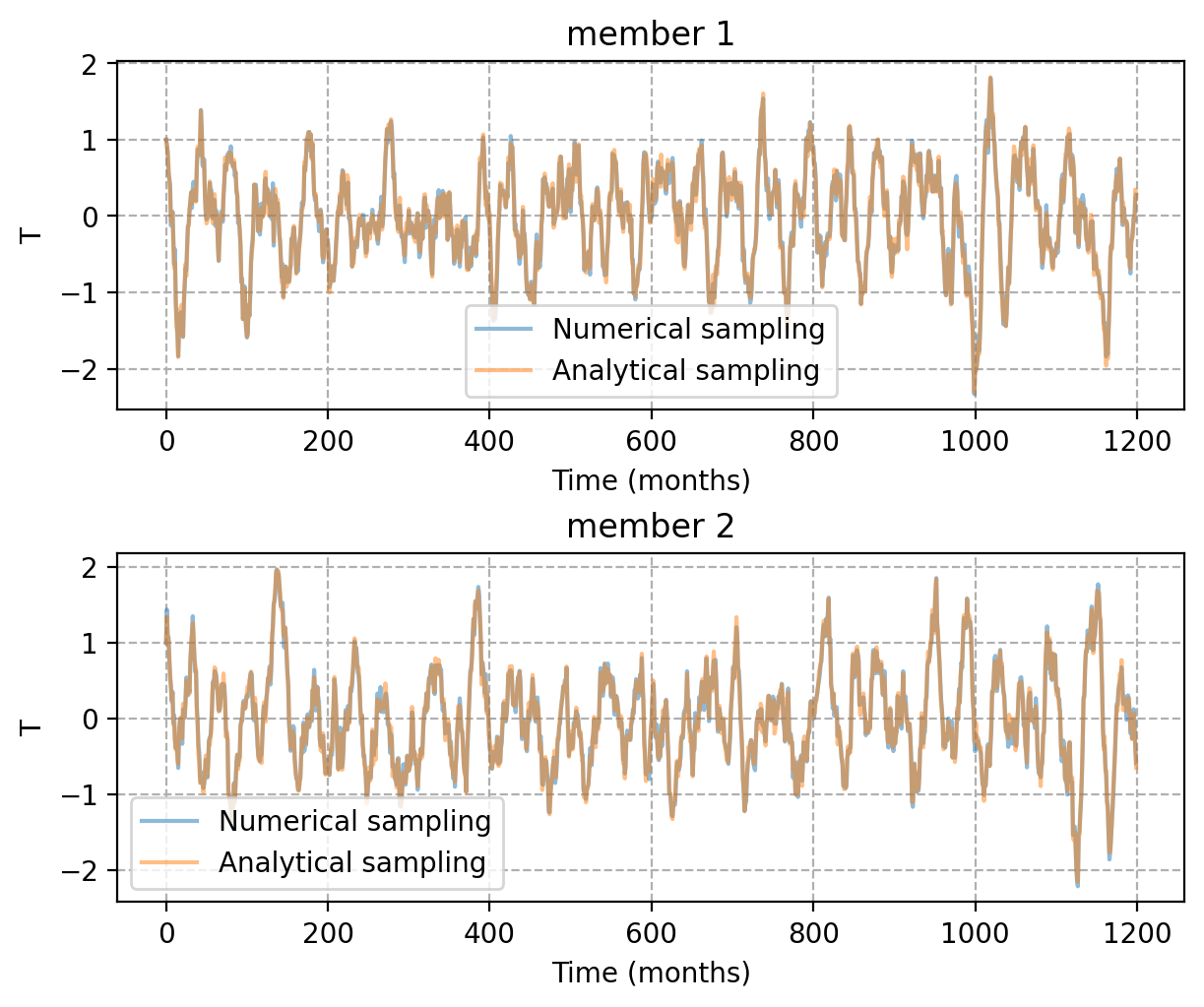
This function returns the analytical solution for the linear RO system without seasonality, using white additive noise.

Its usage is structurally similar to RO_solver, but with the following key differences: 'NM' (numerical method) and 'EF' (external forcing) are not required or accepted.
To ensure a meaningful comparison with the numerical solution from RO_solver, use the same seed for noise_custom in both simulations.

[8]:

# Example 3-3. Compare numerical and analyticla solution
NE = 2
T_ro, h_ro, _ = pyCRO.RO_solver(par, IC, N, NE, NM, dt, saveat, savemethod, EF, noise_custom)
T_ref, h_ref, _ = pyCRO.RO_analytic_solver(par, IC, N, NE, dt, saveat, savemethod, noise_custom)

time_axis = np.arange(0, N, saveat)

fig, axes = plt.subplots(2, 1, figsize=(6, 5), layout='compressed')
for i, ax in enumerate(axes.flat):
    ax.plot(time_axis, T_ro[:, i],  label='Numerical sampling',  alpha=0.5)
    ax.plot(time_axis, T_ref[:, i], label='Analytical sampling', alpha=0.5)
    ax.set_xlabel("Time (months)")
    ax.set_ylabel("T")
    ax.legend()
    ax.grid(ls='--')
    ax.set_title(f"member {i+1}")

---------------------------------------------------------------------------------
Welcome to the CRO Solver! Your simulation setup is as follows:
---------------------------------------------------------------------------------
 - Total simulation length: N = 1200 months
 - Number of ensemble members: NE = 2
 - Numerical integration time step: dt = 0.1 months (default: 0.1)
 - Data output interval: saveat = 1.0 months (default: 1.0)
 - Initial conditions: IC = [T0, h0] = [1.0, 0.0]
 - Input parameters have the expected shapes.
 - 'n_T' = 1: White noise forcing in T; 'm_T' ignored.
 - 'n_h' = 1: White noise forcing in h; 'm_h' ignored.
 - 'n_g' = 2: Additive noise is used in the T equation; 'B' is ignored.
 - Numerical integration method: NM = 'EH' (Euler–Heun method; default)
 - Data saving method: savemethod = sampling (default)
 - External forcing is not given, therefore using
   EF = {'E_T': [0.0, 0.0, 0.0, 0.0, 0.0], 'E_h': [0.0, 0.0, 0.0, 0.0, 0.0]}.
 - noise_custom = 999: seeded same noise.
---------------------------------------------------------------------------------
Numerical integration starting:
---------------------------------------------------------------------------------
---------------------------------------------------------------------------------
All steps successfully completed!
---------------------------------------------------------------------------------
---------------------------------------------------------------------------------
Welcome to the CRO Analytical Solver!
Ensure that the same arguments are provided as for RO_solver,
 except that 'NM' and 'EF' are not required.
---------------------------------------------------------------------------------
All steps are successfully completed!
---------------------------------------------------------------------------------

Analytical Amplitude of RO#

``pyCRO.RO_analytic_std(par)``

It returns the theoretical standard deviations for the linear-white-additive configuration based on the given parameter dictionary par.

``BWJ = pyCRO.RO_BWJ(par)``

It computes the expected BJ and Wyrtki indices, where the real part ({BWJ.real}) corresponds to the BJ index and the imaginary part ({BWJ.imag}) corresponds to the Wyrtki index, based on the given parameter dictionary par.

[9]:

# Example 3-4. Compare standard deviation of numerical and analytial solutions
T_ref_std, h_ref_std = pyCRO.RO_analytic_std(par) # calculate theoretical standard deviations

T_ro, h_ro, _ = pyCRO.RO_solver(par, IC, N, NE, NM, dt, saveat, savemethod, noise_custom=None)
T_ro_std = np.std(T_ro, axis=0); h_ro_std = np.std(h_ro, axis=0)
T_ro_std_mean = np.mean(T_ro_std); h_ro_std_mean = np.mean(h_ro_std) # ensemble mean

print("Standard drviations for T (analytical):")
print(T_ref_std)
print("Standard drviations for T (ensemble mean for numerical solutions):")
print(T_ro_std_mean)
print("Standard drviations for h (analytical):")
print(h_ref_std)
print("Standard drviations for h (ensemble mean for numerical solutions):")
print(h_ro_std_mean)

# Example 3-5. Calculate BWJ Index

BWJ = pyCRO.RO_BWJ(par)
print(f"BJ index: {BWJ.real} [1/month]")
print(f"Wyrtki index: {BWJ.imag:.3f} [1/month]. "
      f"This corresponds to a periodicity of {2*np.pi/BWJ.imag:.3f} months.")

---------------------------------------------------------------------------------
Welcome to the CRO Solver! Your simulation setup is as follows:
---------------------------------------------------------------------------------
 - Total simulation length: N = 1200 months
 - Number of ensemble members: NE = 2
 - Numerical integration time step: dt = 0.1 months (default: 0.1)
 - Data output interval: saveat = 1.0 months (default: 1.0)
 - Initial conditions: IC = [T0, h0] = [1.0, 0.0]
 - Input parameters have the expected shapes.
 - 'n_T' = 1: White noise forcing in T; 'm_T' ignored.
 - 'n_h' = 1: White noise forcing in h; 'm_h' ignored.
 - 'n_g' = 2: Additive noise is used in the T equation; 'B' is ignored.
 - Numerical integration method: NM = 'EH' (Euler–Heun method; default)
 - Data saving method: savemethod = sampling (default)
 - External forcing is not given, therefore using
   EF = {'E_T': [0.0, 0.0, 0.0, 0.0, 0.0], 'E_h': [0.0, 0.0, 0.0, 0.0, 0.0]}.
 - noise_custom = None: System-generated noise is used and changes at every run.
---------------------------------------------------------------------------------
Numerical integration starting:
---------------------------------------------------------------------------------
---------------------------------------------------------------------------------
All steps successfully completed!
---------------------------------------------------------------------------------
Standard drviations for T (analytical):
0.6679474875720741
Standard drviations for T (ensemble mean for numerical solutions):
0.6661314788743359
Standard drviations for h (analytical):
4.531937945124749
Standard drviations for h (ensemble mean for numerical solutions):
4.610590240926273
BJ index: -0.04 [1/month]
Wyrtki index: 0.134 [1/month]. This corresponds to a periodicity of 46.963 months.

RO simulations using CRO solver#