`CRO` fitting with CMIP6 models#

This tutorial illustrates how to use the pyCRO to estimate RO parameters from all CMIP6 models

Contact:

Sen Zhao (zhaos@hawaii.edu)

Load library#

[1]:

%config IPCompleter.greedy = True
%matplotlib inline
%config InlineBackend.figure_format='retina'

%load_ext autoreload
%autoreload 2

import os
import sys

import numpy as np
import xarray as xr
import matplotlib.pyplot as plt

## comment this if you install pyCRO already
sys.path.append(os.path.abspath("../../../"))

import pyCRO

Fitting RO to the all CMIP6 models#

[3]:

def fit_dict_to_dataset(fit_dict):
    """
    Convert a single fit dictionary into an xarray.Dataset.
    Assigns dimensions based on the length of the parameter list:
        len=1 -> 'ac_0'
        len=3 -> 'ac_1'
        len=5 -> 'ac_2'
    Empty lists are replaced with np.nan (float).

    Parameters
    ----------
    fit_dict : dict
        Dictionary where keys are parameter names and values are lists.

    Returns
    -------
    xr.Dataset
    """
    data_vars = {}

    for k, v in fit_dict.items():
        if len(v) == 0:
            arr = np.array([np.nan], dtype=float)
            dim = "ac_0"
        elif len(v) == 1:
            arr = np.array(v, dtype=float)
            dim = "ac_0"
        elif len(v) == 3:
            arr = np.array(v, dtype=float)
            dim = "ac_1"
        elif len(v) == 5:
            arr = np.array(v, dtype=float)
            dim = "ac_2"
        else:
            # Other lengths: convert to float, pad with nan if needed
            arr = np.array(v, dtype=float)
            dim = f"ac_{len(v)}"

        data_vars[k] = (dim, arr)

    return xr.Dataset(data_vars)


def CRO_cmip6_fitting(par_option_T, par_option_h, par_option_noise, verbose=False):
    """
        fit all cmip6 models with the same T, h, and noise options
    """

    for i, model in enumerate(cmip_ds.model.values):
        par_tmp = pyCRO.RO_fitting(cmip_ds['Nino34'].sel(model=model), cmip_ds['Hm'].sel(model=model),
                                   par_option_T, par_option_h, par_option_noise, verbose=verbose)
        par_ds = fit_dict_to_dataset(par_tmp).assign_coords({'model': model})

        if i==0:
            par_cmip = par_ds
        else:
            par_cmip = xr.concat([par_cmip, par_ds], dim='model')
    return par_cmip

Understanding relationship between ENSO amplitude and RO parameters#

Calculation of seasonal variance

[6]:

cmip_SD = cmip_ds['Nino34'].var('time')

[7]:

fig, axes = plt.subplots(1, 2, figsize=(8, 4), sharey=True, layout='compressed')

ax = axes[0]
ax.scatter((par_cmip_LWA['R']-par_cmip_LWA['epsilon'])*0.5, cmip_SD, label='Linear RO')
ax.scatter((par_cmip_NWA['R']-par_cmip_NWA['epsilon'])*0.5, cmip_SD, label='Nonlinear RO')
ax.set_xlabel('BJ (month$^{-1}$)')
ax.set_ylabel(r"Nino34 index variance (K$^2$)")
ax.legend(fontsize=9)

ax = axes[1]
ax.scatter(par_cmip_LWA['sigma_T'], cmip_SD, label='Linear RO')
ax.scatter(par_cmip_NWA['sigma_T'], cmip_SD, label='Nonlinear RO')
ax.set_xlabel(r"$\sigma_T$ (K month$^{-1/2}$)")

[7]:

Text(0.5, 0, '$\\sigma_T$ (K month$^{-1/2}$)')

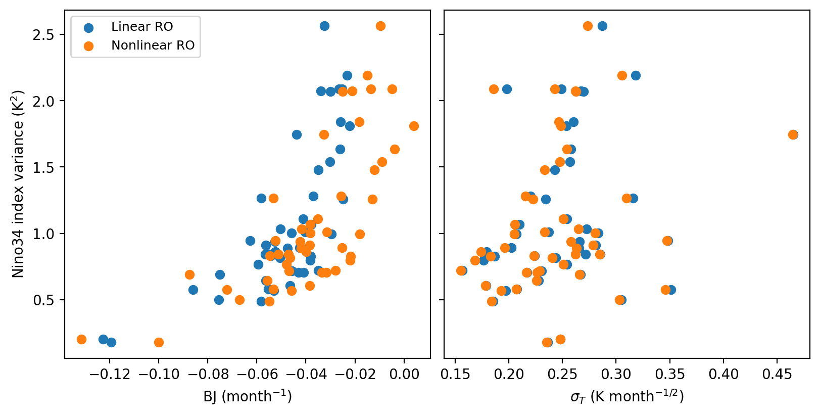
../_images/notebooks_fitting_cmip6_14_1.png

The ENSO amplitude is highly related the growth rate (BJ index) and a less degree to noise amplitude.