`CRO` fitting with observation#

This tutorial illustrates how to use the pyCRO to estimate RO parameters from the observations

Contact:

Sen Zhao (zhaos@hawaii.edu)

Load library#

[1]:

%config IPCompleter.greedy = True
%matplotlib inline
%config InlineBackend.figure_format='retina'

%load_ext autoreload
%autoreload 2

import os
import sys

import numpy as np
import xarray as xr
import matplotlib.pyplot as plt

## comment this if you install pyCRO already
sys.path.append(os.path.abspath("../../../"))

import pyCRO

[2]:

pyCRO.RO_fitting?

Signature:
pyCRO.RO_fitting(
    T,
    h,
    par_option_T,
    par_option_h,
    par_option_noise,
    method_fitting=None,
    dt=None,
    verbose=True,
)
Docstring:
Fit the Recharge Oscillator (RO) model parameters to T and h time series.

This function performs parameter fitting for the RO system, using the specified
prescribed parameter options and noise characteristics. Fitting can be done
via linear regression (LR) or maximum likelihood estimation (MLE), with optional
handling for multiplicative or additive noise. It can automatically select a
default fitting method based on parameter options.

Parameters
----------
T : ndarray
    Time series of SST anomalies (1D array).
h : ndarray
    Time series of thermocline anomalies (1D array).
par_option_T : dict
    Prescribed options for SST equation parameters.
par_option_h : dict
    Prescribed options for thermocline equation parameters.
par_option_noise : dict
    Noise settings, e.g., {'T': 'red', 'h': 'red', 'T_type': 'multiplicative'}.
method_fitting : str, optional
    Fitting method to use: 'LR-F', 'LR-C', 'LR-F-MAC', or 'MLE'.
    If None, the method is determined automatically.
dt : float, optional
    Time step of the input time series. Default is 1.0 (months).
verbose : bool, optional
    If True, prints fitting information and progress.

Returns
-------
dict
    Dictionary of fitted CRO parameters:
    Keys include:
    'R', 'F1', 'F2', 'epsilon', 'b_T', 'c_T', 'd_T', 'b_h',
    'sigma_T', 'sigma_h', 'B', 'm_T', 'm_h', 'n_T', 'n_h', 'n_g'.

Notes
-----
- Automatically removes mean from input time series.
- Applies Ito-to-Stratonovich correction for multiplicative noise.
- Negligible seasonal amplitudes are rounded to zero.
- Ensures consistent noise settings for T and h equations.
- Prints a summary of the fitting process if `verbose` is True.

Examples
--------
>>> par_option_T = {'mean': 1, 'seasonal': 3, 'semi_annual': 0, ...}
>>> par_option_h = {'mean': 1, 'seasonal': 3, 'semi_annual': 0, ...}
>>> par_option_noise = {'T': 'red', 'h': 'red', 'T_type': 'multiplicative'}
>>> fitted_params = RO_fitting(T, h, par_option_T, par_option_h, par_option_noise)
>>> print(fitted_params['sigma_T'])
File:      ~/codes/CRO/pyCRO/fitting.py
Type:      function

RO Parameter Fitting Usage#

``par_fitted = pyCRO.RO_fitting(T, h, par_option_T, par_option_h, par_option_noise)``

Input T and h Time Series#

T and h are input timeseries used for the fitting.
T and h must be 1D time series arrays with a uniform time step.

Specifiying RO Type#

These options define the RO model type used for fitting.

par_option_T specifies the linear and nonlinear terms in dT/dt
par_option_h specifies the linear and nonlinear terms in dh/dt
par_option_noise specifies the noise type

The following example shows how to set the RO type as linear-white-additive RO for the fitting.

par_option_T = {"R": 1, "F1": 1, "b_T": 0, "c_T": 0, "d_T": 0}
par_option_h = {"F2": 1, "epsilon": 1, "b_h": 0}

For keys in par_option_T and par_option_h, allowed values are:
- 0 — Do not estimate
- 1 — Estimate only the annual mean
- 3 — Estimate annual mean + annual seasonality
- 5 — Estimate annual mean + annual + semi-annual seasonality

par_option_noise = {"T": "white", "h": "white", "T_type": "multiplicative"}

Valid options for \(T\) and \(h\) are:
- "white": white noise forcing
- "red": red noise forcing
Both \(T\) and \(h\) must use the same noise type; otherwise, an error is raised.
Valid options for T-type (noise structure for \(T\)) are:
- "additive": T noise forcing is additive
- "multiplicative": T noise forcing is multiplicative
- "multiplicative-H": T noise forcing is Heaviside based-multiplicative noise

Fitting RO to the observation/reanalysis#

Load observed ENSO timeseries from ORAS5#

[3]:

# load observations
file_name = os.path.join(os.getcwd(), "../../../data", "XRO_indices_oras5.nc")
xr_ds = xr.open_dataset(file_name)
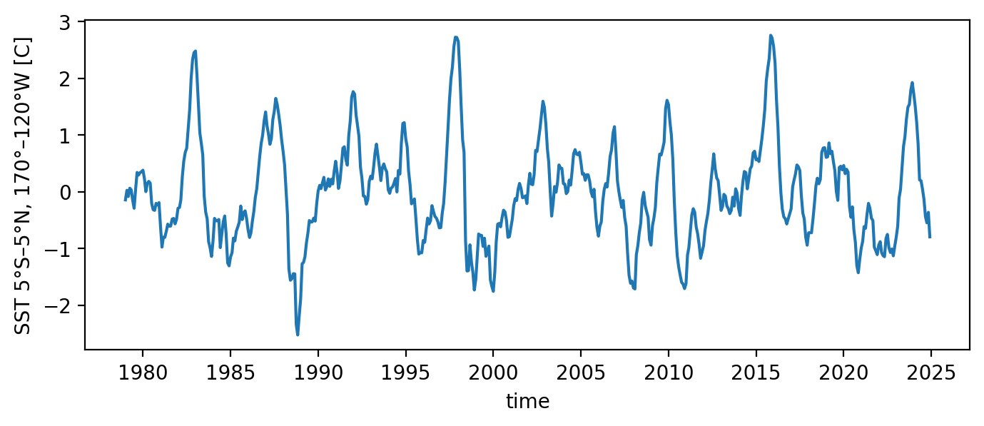
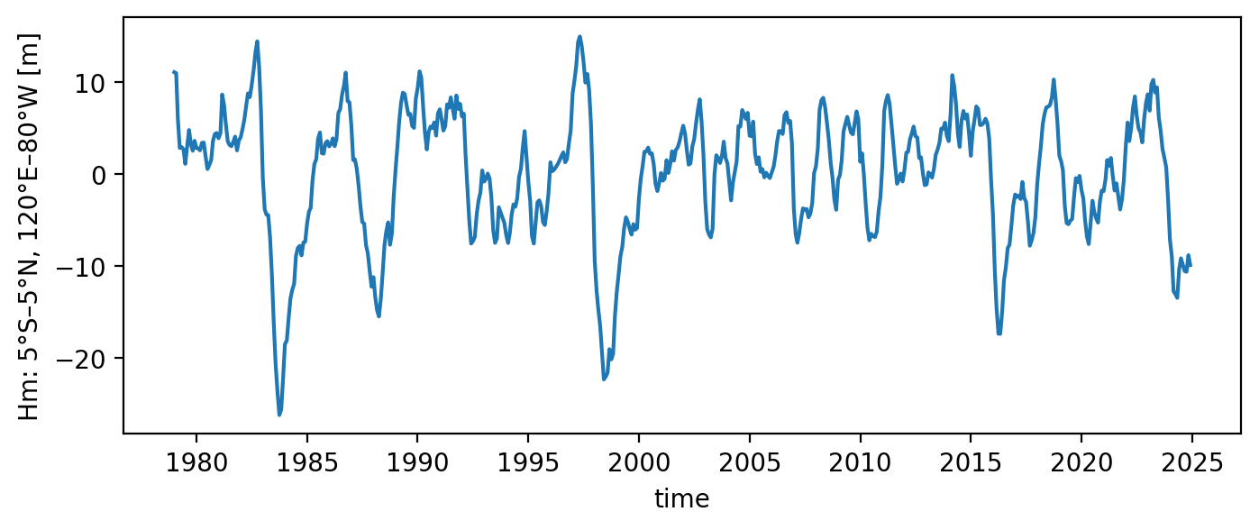
T_oras5 = xr_ds['Nino34'][:]  # Nino 3.4 since 1979-01-01
h_oras5 = xr_ds['WWV'][:]     # WWV since 1979-01-01
time_oras5 = xr_ds['time'][:] # Days since 1979-01-01

T_oras5.plot(figsize=(8, 3))
h_oras5.plot(figsize=(8, 3))

[3]:

[<matplotlib.lines.Line2D at 0x15466d310>]

../_images/notebooks_fitting_obs_7_1.png

../_images/notebooks_fitting_obs_7_2.png

Type Linear-White-Additive#

Fit linear RO with white and additive noise

[4]:

par_option_T = {"R": 1, "F1": 1, "b_T": 0, "c_T": 0, "d_T": 0}
par_option_h = {"F2": 1, "epsilon": 1, "b_h": 0}
par_option_noise = {"T": "white", "h": "white", "T_type": "additive"}

par_obs_LWA = pyCRO.RO_fitting(T_oras5, h_oras5, par_option_T, par_option_h, par_option_noise)
par_obs_LWA

---------------------------------------------------------------------------------
Welcome to CRO Fitting! Your fitting setups:
---------------------------------------------------------------------------------
 - Data time step is not given, defaulting to: dt = 1.0 months.
 - Time series length: N = len(T)*dt = 552.0 months.
 - Prescribed terms: {'R': 1, 'F1': 1, 'b_T': 0, 'c_T': 0, 'd_T': 0}.
                     {'F2': 1, 'epsilon': 1, 'b_h': 0}.
   0 - Do not prescribe.
   1 - Prescribe only the annual mean.
   3 - Prescribe the annual mean and annual seasonality.
   5 - Prescribe the annual mean, annual seasonality, and semi-annual seasonality.
 - Noise options: {'T': 'white', 'h': 'white', 'T_type': 'additive'}.
 - Fitting method for T and h main equations: None.
Referring to table_default_fitting_method.txt and using LR-F
---------------------------------------------------------------------------------
All steps are successfully completed!
---------------------------------------------------------------------------------

[4]:

{'R': [-0.07438421424913766],
 'F1': [0.01933022284607733],
 'F2': [1.2506110930680376],
 'epsilon': [0.005104133449149751],
 'b_T': [],
 'c_T': [],
 'd_T': [],
 'b_h': [],
 'sigma_T': [0.22171941830446124],
 'sigma_h': [1.6039500028588676],
 'B': [],
 'm_T': [],
 'm_h': [],
 'n_T': [1],
 'n_h': [1],
 'n_g': [2]}

Type Seasonal-Linear-White-Additive#

Fit seasonal linear RO with white and additive noise

[5]:

par_option_T = {"R": 3, "F1": 3, "b_T": 0, "c_T": 0, "d_T": 0}
par_option_h = {"F2": 3, "epsilon": 3, "b_h": 0}
par_option_noise = {"T": "white", "h": "white", "T_type": "additive"}

par_obs_SLWA = pyCRO.RO_fitting(T_oras5, h_oras5, par_option_T, par_option_h, par_option_noise)
par_obs_SLWA

---------------------------------------------------------------------------------
Welcome to CRO Fitting! Your fitting setups:
---------------------------------------------------------------------------------
 - Data time step is not given, defaulting to: dt = 1.0 months.
 - Time series length: N = len(T)*dt = 552.0 months.
 - Prescribed terms: {'R': 3, 'F1': 3, 'b_T': 0, 'c_T': 0, 'd_T': 0}.
                     {'F2': 3, 'epsilon': 3, 'b_h': 0}.
   0 - Do not prescribe.
   1 - Prescribe only the annual mean.
   3 - Prescribe the annual mean and annual seasonality.
   5 - Prescribe the annual mean, annual seasonality, and semi-annual seasonality.
 - Noise options: {'T': 'white', 'h': 'white', 'T_type': 'additive'}.
 - Fitting method for T and h main equations: None.
Referring to table_default_fitting_method.txt and using LR-F
---------------------------------------------------------------------------------
All steps are successfully completed!
---------------------------------------------------------------------------------

[5]:

{'R': [-0.05593351982606123, 0.15313660361276363, -2.737173916414297],
 'F1': [0.013718888027663807, 0.009846162690394499, -0.9042975099904762],
 'F2': [1.1291210149159407, 0.8323142760801497, 1.061471770708532],
 'epsilon': [0.023584768568800617, 0.03920999829130576, 0.2619998710028356],
 'b_T': [],
 'c_T': [],
 'd_T': [],
 'b_h': [],
 'sigma_T': [0.2010388126198346],
 'sigma_h': [1.5036959788770163],
 'B': [],
 'm_T': [],
 'm_h': [],
 'n_T': [1],
 'n_h': [1],
 'n_g': [2]}

Type Seasonal-Nonlinear-White-Additive#

Fit seasonal nonlinear RO with white and additive noise

[6]:

par_option_T = {"R": 3, "F1": 3, "b_T": 3, "c_T": 3, "d_T": 3}
par_option_h = {"F2": 3, "epsilon": 3, "b_h": 3}
par_option_noise = {"T": "white", "h": "white", "T_type": "additive"}

par_obs_SNWA = pyCRO.RO_fitting(T_oras5, h_oras5, par_option_T, par_option_h, par_option_noise)
par_obs_SNWA

---------------------------------------------------------------------------------
Welcome to CRO Fitting! Your fitting setups:
---------------------------------------------------------------------------------
 - Data time step is not given, defaulting to: dt = 1.0 months.
 - Time series length: N = len(T)*dt = 552.0 months.
 - Prescribed terms: {'R': 3, 'F1': 3, 'b_T': 3, 'c_T': 3, 'd_T': 3}.
                     {'F2': 3, 'epsilon': 3, 'b_h': 3}.
   0 - Do not prescribe.
   1 - Prescribe only the annual mean.
   3 - Prescribe the annual mean and annual seasonality.
   5 - Prescribe the annual mean, annual seasonality, and semi-annual seasonality.
 - Noise options: {'T': 'white', 'h': 'white', 'T_type': 'additive'}.
 - Fitting method for T and h main equations: None.
Referring to table_default_fitting_method.txt and using LR-F
---------------------------------------------------------------------------------
All steps are successfully completed!
---------------------------------------------------------------------------------

[6]:

{'R': [-0.0382566265025694, 0.1527926109826267, -2.6649612100849693],
 'F1': [0.014880562268928867, 0.009087329130650648, -1.0317328769740488],
 'F2': [1.0869104940931082, 0.836138603016686, 0.9978616403641565],
 'epsilon': [0.02686761171394466, 0.03811643856137869, 0.3515145112713374],
 'b_T': [0.015496318456175271, 0.02172909602605961, 0.15331563818664037],
 'c_T': [0.011128872374761921, 0.007610249369034017, -1.4816355854434864],
 'd_T': [0.00836643586808151, 0.004079034223791854, -1.4009025018867796],
 'b_h': [0.07951113081904435, 0.06548708161774483, 2.7744417360145204],
 'sigma_T': [0.19385539074789102],
 'sigma_h': [1.4970166742429747],
 'B': [],
 'm_T': [],
 'm_h': [],
 'n_T': [1],
 'n_h': [1],
 'n_g': [2]}

Type Seasonal-Nonlinear-Red-Additive#

Fit seasonal nonlinear RO with red and additive noise

[7]:

par_option_T = {"R": 3, "F1": 3, "b_T": 3, "c_T": 3, "d_T": 3}
par_option_h = {"F2": 3, "epsilon": 3, "b_h": 3}
par_option_noise = {"T": "red", "h": "red", "T_type": "additive"}

par_obs_SNRA = pyCRO.RO_fitting(T_oras5, h_oras5, par_option_T, par_option_h, par_option_noise)
par_obs_SNRA

---------------------------------------------------------------------------------
Welcome to CRO Fitting! Your fitting setups:
---------------------------------------------------------------------------------
 - Data time step is not given, defaulting to: dt = 1.0 months.
 - Time series length: N = len(T)*dt = 552.0 months.
 - Prescribed terms: {'R': 3, 'F1': 3, 'b_T': 3, 'c_T': 3, 'd_T': 3}.
                     {'F2': 3, 'epsilon': 3, 'b_h': 3}.
   0 - Do not prescribe.
   1 - Prescribe only the annual mean.
   3 - Prescribe the annual mean and annual seasonality.
   5 - Prescribe the annual mean, annual seasonality, and semi-annual seasonality.
 - Noise options: {'T': 'red', 'h': 'red', 'T_type': 'additive'}.
 - Fitting method for T and h red noises: ARn.
   This option is defined internally within fit.py.
   Options available are: LR or AR1 or ARn.
 - Fitting method for T and h main equations: None.
Referring to table_default_fitting_method.txt and using LR-F
---------------------------------------------------------------------------------
All steps are successfully completed!
---------------------------------------------------------------------------------

[7]:

{'R': [-0.0382566265025694, 0.1527926109826267, -2.6649612100849693],
 'F1': [0.014880562268928867, 0.009087329130650648, -1.0317328769740488],
 'F2': [1.0869104940931082, 0.836138603016686, 0.9978616403641565],
 'epsilon': [0.02686761171394466, 0.03811643856137869, 0.3515145112713374],
 'b_T': [0.015496318456175271, 0.02172909602605961, 0.15331563818664037],
 'c_T': [0.011128872374761921, 0.007610249369034017, -1.4816355854434864],
 'd_T': [0.00836643586808151, 0.004079034223791854, -1.4009025018867796],
 'b_h': [0.07951113081904435, 0.06548708161774483, 2.7744417360145204],
 'sigma_T': [0.19385539074789102],
 'sigma_h': [1.4970166742429747],
 'B': [],
 'm_T': [1.7019681249729073],
 'm_h': [1.6733758118727624],
 'n_T': [0],
 'n_h': [0],
 'n_g': [2]}

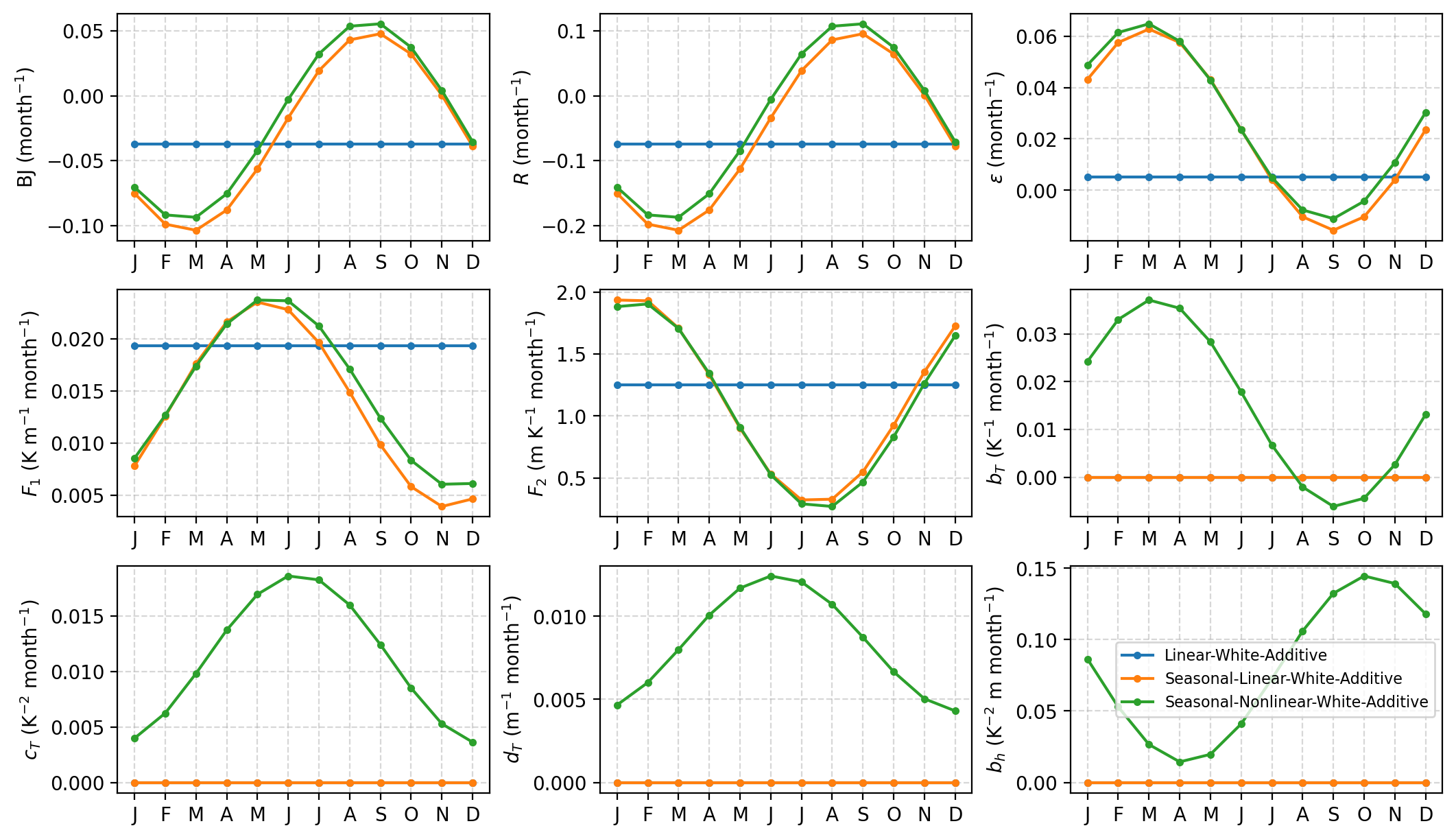
Visualize the deterministic RO parameters#

[8]:

axes = pyCRO.plot_RO_par(par_obs_LWA, label='Linear-White-Additive', ncol=3)
axes = pyCRO.plot_RO_par(par_obs_SLWA, label='Seasonal-Linear-White-Additive', ncol=3, ax=axes)
axes = pyCRO.plot_RO_par(par_obs_SNWA, label='Seasonal-Nonlinear-White-Additive', ncol=3, ax=axes)
axes[-1].legend(fontsize=8)

[8]:

<matplotlib.legend.Legend at 0x10977f560>

../_images/notebooks_fitting_obs_17_1.png

Simulating ENSO with observed RO parameters#

[9]:

def CRO_simulate(par, IC=[0, 0], N=12*200, NE=100, verbose=False):
    """
        CRO simulation (solver) with defined parameters

            default: 100 member with 200 yrs each member
    """
    T_out, h_out, noise_out = pyCRO.RO_solver(par, IC=IC, N=N, NE=NE, verbose=verbose)
    xtime = xr.date_range('0001-01', periods=N, freq = 'MS', use_cftime=True)
    member = np.arange(0, NE, step=1)
    T_ds = xr.DataArray(T_out, dims={'time', 'member'}, coords={'time': xtime, 'member': member})
    h_ds = xr.DataArray(h_out, dims={'time', 'member'}, coords={'time': xtime, 'member': member})
    RO_ds = xr.Dataset({'Nino34': T_ds, 'WWV': h_ds})
    return RO_ds

simulation with LWA type#

[10]:

%%time
RO_obs_LWA = CRO_simulate(par_obs_LWA, verbose=True)

---------------------------------------------------------------------------------
Welcome to the CRO Solver! Your simulation setup is as follows:
---------------------------------------------------------------------------------
 - Total simulation length: N = 2400 months
 - Number of ensemble members: NE = 100
 - Numerical integration time step: dt = 0.1 months (default: 0.1)
 - Data output interval: saveat = 1.0 months (default: 1.0)
 - Initial conditions: IC = [T0, h0] = [0, 0]
 - Input parameters have the expected shapes.
 - 'n_T' = 1: White noise forcing in T; 'm_T' ignored.
 - 'n_h' = 1: White noise forcing in h; 'm_h' ignored.
 - 'n_g' = 2: Additive noise is used in the T equation; 'B' is ignored.
 - Numerical integration method: NM = 'EH' (Euler–Heun method; default)
 - Data saving method: savemethod = sampling (default)
 - External forcing is not given, therefore using
   EF = {'E_T': [0.0, 0.0, 0.0, 0.0, 0.0], 'E_h': [0.0, 0.0, 0.0, 0.0, 0.0]}.
 - noise_custom = None: System-generated noise is used and changes at every run.
---------------------------------------------------------------------------------
Numerical integration starting:
---------------------------------------------------------------------------------
---------------------------------------------------------------------------------
All steps successfully completed!
---------------------------------------------------------------------------------
CPU times: user 2.12 s, sys: 56.5 ms, total: 2.17 s
Wall time: 2.18 s

[11]:

%%time

RO_obs_SLWA = CRO_simulate(par_obs_SLWA, verbose=False)
RO_obs_SNWA = CRO_simulate(par_obs_SNWA, verbose=False)
RO_obs_SNRA = CRO_simulate(par_obs_SNRA, verbose=False)

CPU times: user 6.62 s, sys: 69.3 ms, total: 6.69 s
Wall time: 6.69 s

calculation of seasonal standard deivation

[12]:

%%time

seaSD_obs = xr_ds.groupby('time.month').std('time')
seaSD_obsRO_LWA = RO_obs_LWA.groupby('time.month').std('time')
seaSD_obsRO_SLWA = RO_obs_SLWA.groupby('time.month').std('time')
seaSD_obsRO_SNWA = RO_obs_SNWA.groupby('time.month').std('time')
seaSD_obsRO_SNRA = RO_obs_SNRA.groupby('time.month').std('time')

CPU times: user 55.1 ms, sys: 7.33 ms, total: 62.4 ms
Wall time: 64.4 ms

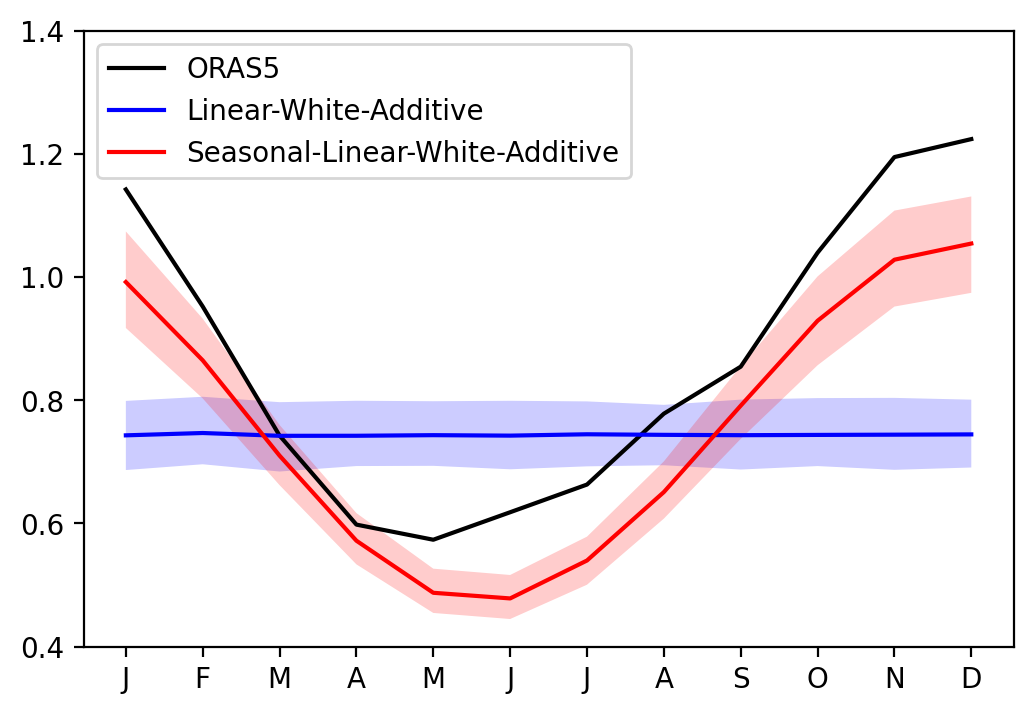
Effect of seasonal cycle of RO linear parameters#

[13]:

sel_var = 'Nino34'

fig, ax = plt.subplots(1, 1, figsize=(6, 4))

ax.plot(seaSD_obs.month, seaSD_obs[sel_var], c='k', label='ORAS5')

ax.plot(seaSD_obsRO_LWA.month, seaSD_obsRO_LWA[sel_var].mean('member'), c='blue', label='Linear-White-Additive')
ax.fill_between(seaSD_obsRO_LWA.month, seaSD_obsRO_LWA[sel_var].quantile(0.1, dim='member'), seaSD_obsRO_LWA[sel_var].quantile(0.9, dim='member'), fc='blue', alpha=0.2)

ax.plot(seaSD_obsRO_SLWA.month, seaSD_obsRO_SLWA[sel_var].mean('member'), c='red', label='Seasonal-Linear-White-Additive')
ax.fill_between(seaSD_obsRO_SLWA.month, seaSD_obsRO_SLWA[sel_var].quantile(0.1, dim='member'), seaSD_obsRO_SLWA[sel_var].quantile(0.9, dim='member'), fc='red', alpha=0.2)

ax.set_xticks(range(1, 13))
ax.set_xticklabels(["J","F","M","A","M","J","J","A","S","O","N","D"])
ax.set_ylim([0.4, 1.4])
ax.legend()

[13]:

<matplotlib.legend.Legend at 0x1546e30e0>

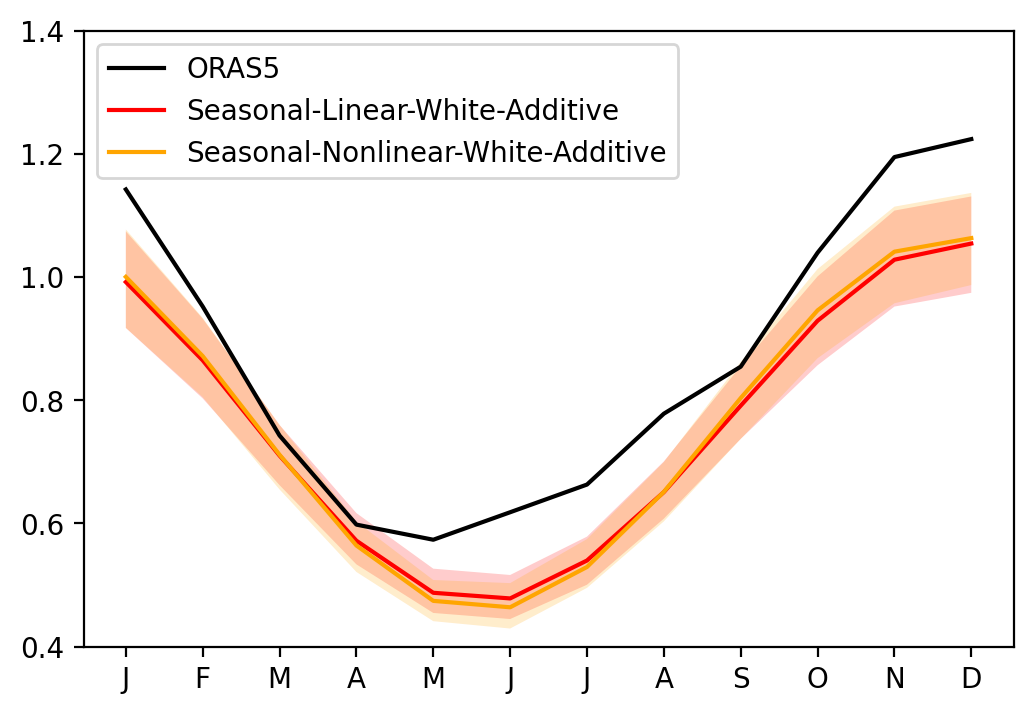
../_images/notebooks_fitting_obs_26_1.png

Effect of RO nonlinear parameters#

[14]:

sel_var = 'Nino34'

fig, ax = plt.subplots(1, 1, figsize=(6, 4))

ax.plot(seaSD_obs.month, seaSD_obs[sel_var], c='k', label='ORAS5')

ax.plot(seaSD_obsRO_SLWA.month, seaSD_obsRO_SLWA[sel_var].mean('member'), c='red', label='Seasonal-Linear-White-Additive')
ax.fill_between(seaSD_obsRO_SLWA.month, seaSD_obsRO_SLWA[sel_var].quantile(0.1, dim='member'), seaSD_obsRO_SLWA[sel_var].quantile(0.9, dim='member'), fc='red', alpha=0.2)

ax.plot(seaSD_obsRO_SNWA.month, seaSD_obsRO_SNWA[sel_var].mean('member'), c='orange', label='Seasonal-Nonlinear-White-Additive')
ax.fill_between(seaSD_obsRO_SNWA.month, seaSD_obsRO_SNWA[sel_var].quantile(0.1, dim='member'), seaSD_obsRO_SNWA[sel_var].quantile(0.9, dim='member'), fc='orange', alpha=0.2)

ax.set_xticks(range(1, 13))
ax.set_xticklabels(["J","F","M","A","M","J","J","A","S","O","N","D"])
ax.set_ylim([0.4, 1.4])
ax.legend()

[14]:

<matplotlib.legend.Legend at 0x157c72810>

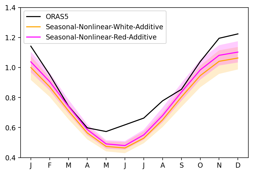
../_images/notebooks_fitting_obs_28_1.png

Red noise vs White noise#

[15]:

sel_var = 'Nino34'

fig, ax = plt.subplots(1, 1, figsize=(6, 4))

ax.plot(seaSD_obs.month, seaSD_obs[sel_var], c='k', label='ORAS5')

ax.plot(seaSD_obsRO_SNWA.month, seaSD_obsRO_SNWA[sel_var].mean('member'), c='orange', label='Seasonal-Nonlinear-White-Additive')
ax.fill_between(seaSD_obsRO_SNWA.month, seaSD_obsRO_SNWA[sel_var].quantile(0.1, dim='member'), seaSD_obsRO_SNWA[sel_var].quantile(0.9, dim='member'), fc='orange', alpha=0.2)

ax.plot(seaSD_obsRO_SNRA.month, seaSD_obsRO_SNRA[sel_var].mean('member'), c='magenta', label='Seasonal-Nonlinear-Red-Additive')
ax.fill_between(seaSD_obsRO_SNRA.month, seaSD_obsRO_SNRA[sel_var].quantile(0.1, dim='member'), seaSD_obsRO_SNRA[sel_var].quantile(0.9, dim='member'), fc='magenta', alpha=0.2)

ax.set_xticks(range(1, 13))
ax.set_xticklabels(["J","F","M","A","M","J","J","A","S","O","N","D"])
ax.set_ylim([0.4, 1.4])
ax.legend()

[15]:

<matplotlib.legend.Legend at 0x157d08830>

../_images/notebooks_fitting_obs_30_1.png

Advanced Usage (optional)#

``par_fitted = pyCRO.RO_fitting(T, h, par_option_T, par_option_h, par_option_noise, method_fitting)``

``par_fitted = pyCRO.RO_fitting(T, h, par_option_T, par_option_h, par_option_noise, method_fitting, dt)``

The following block sets additional optional settings for the RO parameter fitting.
The user may skip specifying these options. If the user doesn’t specify these options, the RO parameter fitting runs with the default settings.
method_fitting specifies the parameter fitting method:
- "LR-F": Linear regression (tendency with forward differencing scheme)
- "LR-C": Linear regression (tendency with central differencing scheme)
- "LR-F-MAC": Linear regression (tendency with forward differencing scheme) with Moments Analytical Constraints estimation for T noise parameters
- "MLE": Maximum Likelihood Estimation (tendency with forward differencing scheme)
dt specifies time interval of input T and h time series in month (default = 1.0).
The default method depends on the specified RO type, as indicated in "table_default_fitting_method.txt".
Details of the fitting methods are documented in the manual and the accompanying paper.

[ ]:

CRO fitting with observation#