
Analytical Solutions of the RO Model and Comparison with Numerical Solutions#
This tutorial illustrates how to use the pyCRO to solve the RO model analytically. In Appendix B of CRO paper (Kim et al. in preparation), we derive the analytical solutions for the linear RO model with additive white noise. The system is:
Because the system is linear with additive stochastic forcing, it can be solved using standard methods for linear stochastic differential equations.
Exact time-dependent solutions#
where
and
where:
(\(T_0, h_0\)): initial conditions
(\(w_T, w_h\)): independent white noise processes
(\(\sigma_T, \sigma_h\)): noise amplitudes
Ensemble variance#
Notes#
The system behaves as a damped stochastic oscillator when (4F_1F_2 > (R+:nbsphinx-math:varepsilon)^2).
These analytical expressions provide benchmarks for validating numerical RO solvers in ``pyCRO``.
In practice, stochastic integrals are evaluated using ensemble simulations.
This notebook was contributed by Sen Zhao.
[1]:
%config IPCompleter.greedy = True
%matplotlib inline
%config InlineBackend.figure_format='retina'

%load_ext autoreload
%autoreload 2

import warnings
warnings.filterwarnings("ignore")

import numpy as np
import matplotlib.pyplot as plt
import os
import sys
import calendar

sys.path.append(os.path.abspath("../../../"))

import pyCRO
[6]:
par = {'R': [-0.05],       # dT/dt=R*T (unit: month^-1)
       'F1': [0.02],       # dT/dt=F1*h (unit: K m^-1 month^-1)
       'F2': [0.9],        # dh/dt=-F2*T (unit: m K^-1 month^-1)
       'epsilon': [0.03],  # dh/dt=-epsilon*h (unit: month^-1)
       'b_T': [],          # dT/dt=(b_T)*(T^2) (unit: K^-1 month^-1)
       'c_T': [],          # dT/dt=-(c_T)*(T^3) (unit: K^-2 month^-1)
       'd_T': [],          # dT/dt=(d_T)*(T*h) (unit: m^-1 month^-1)
       'b_h': [],          # dh/dt=-(b_h)*(T^2) (unit: K^-2 m month^-1)
       'sigma_T': [0.2],   # dT/dt=(sigma_T)*(N_T) (unit: K month^-0.5 if n_T=1, K month^-1 if n_T=0)
       'sigma_h': [1.2],   # dh/dt=(sigma_h)*(N_h) (unit: m month^-0.5 if n_h=1, m month^-1 if n_h=0)
       'B': [],            # T/dt=(sigma_T)*(1+B*T)*(N_T) or dT/dt=(sigma_T)*(1+B*H(T)*T)*(N_T) (unit: K^-1)
       'm_T': [],          # d(xi_T)/dt=-m*T*(xi_T); (unit: month^-1)
       'm_h': [],          # d(xi_h)/dt=-m*h*(xi_h); (unit: month^-1)
       'n_T': [1],         # noise type for T (0: red noise, 1: white noise) (unitless)
       'n_h': [1],         # noise type for h (0: red noise, 1: white noise) (unitless)
       'n_g': [2]}         # multiplicative noise type for T (0: linear, 1: Heaviside linear, 2: omit this option)
                           # (note: only valid when B is not zero) (unitless)

IC = [1.0, 0.0]              # Initial conditions for T and h
N = 12 * 100                 # Simulation length in months (e.g., 100 years)
NE = 2                       # Number of ensemble members


NM = "EH"                    # Optional: Numerical integration method for
                             #           RO solver "EH" (Euler–Heun, default)
                             #           or "EM" (Euler–Maruyama)
dt = 0.1                     # Optional: Time step for numerical integration
                             #           in months. Default = 0.1
saveat = 1.0                 # Optional: Interval for saving outputs in months.
                             #           Default = 1.0
savemethod = "sampling"      # Optional: Output method. "sampling" saves
                             #           instantaneous values, "mean" saves
                             #           time-averaged values over each save
                             #           interval. Default = "sampling"
EF = None                    # Optional: External forcing dictionary.
                             #           If EF is None (or not specified),
                             #           it defaults to:
                             #           EF = {'E_T': [0.0], 'E_h': [0.0]}
                             #           Same format and interpretation as
                             #           other RO parameters. Example:
                             #           EF = {'E_T': [-0.01, 0.02, np.pi],
                             #                 'E_h': [-0.01]}
noise_custom = 999           # Optional: Noise specification.
                             #   - If None or not provided:
                             #     uses internally generated noise
                             #     (different each run; Default)
                             #   - If an integer: uses as the random seed for
                             #     reproducible noise with the reference number
                             #   - If ndarray: user-supplied noise
                             #     (shape must be (int(N/dt) - 1, 4))
                             #     The first two columns of the noise array are
                             #     applied to the main T and h equations.
                             #     The last two columns are used as noise terms
                             #     for the red noise processes.
Analytic Solutions of Linear RO With White Noise#
``T_ref, h_ref, _ = pyCRO.RO_analytic_solver(par, IC, N, NE)``
``T_ref, h_ref, _ = pyCRO.RO_analytic_solver(par, IC, N, NE, dt)``
``T_ref, h_ref, _ = pyCRO.RO_analytic_solver(par, IC, N, NE, dt, saveat)``
``T_ref, h_ref, _ = pyCRO.RO_analytic_solver(par, IC, N, NE, dt, saveat, savemethod)``
``T_ref, h_ref, _ = pyCRO.RO_analytic_solver(par, IC, N, NE, dt, saveat, savemethod, noise_custom)``
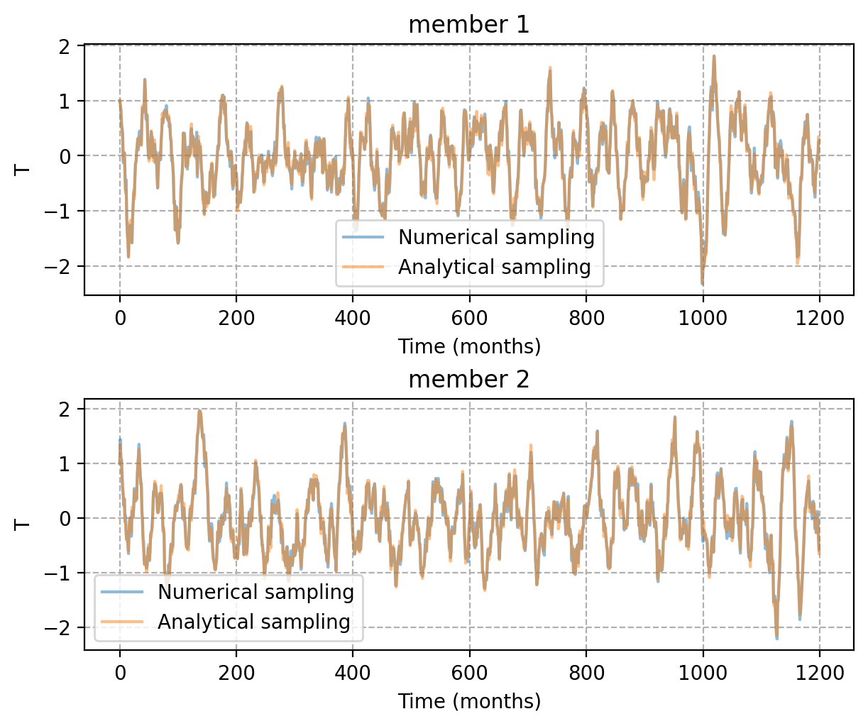
- This function returns the analytical solution for the linear RO system without seasonality, using white additive noise.Its usage is structurally similar to
RO_solver, but with the following key differences:'NM'(numerical method) and'EF'(external forcing) are not required or accepted. To ensure a meaningful comparison with the numerical solution from
RO_solver, use the same seed fornoise_customin both simulations.
[7]:
# Example 3-3. Compare numerical and analyticla solution
NE = 2
T_ro, h_ro, _ = pyCRO.RO_solver(par, IC, N, NE, NM, dt, saveat, savemethod, EF, noise_custom)
T_ref, h_ref, _ = pyCRO.RO_analytic_solver(par, IC, N, NE, dt, saveat, savemethod, noise_custom)

time_axis = np.arange(0, N, saveat)

fig, axes = plt.subplots(2, 1, figsize=(6, 5), layout='compressed')
for i, ax in enumerate(axes.flat):
    ax.plot(time_axis, T_ro[:, i],  label='Numerical sampling',  alpha=0.5)
    ax.plot(time_axis, T_ref[:, i], label='Analytical sampling', alpha=0.5)
    ax.set_xlabel("Time (months)")
    ax.set_ylabel("T")
    ax.legend()
    ax.grid(ls='--')
    ax.set_title(f"member {i+1}")
---------------------------------------------------------------------------------
Welcome to the CRO Solver! Your simulation setup is as follows:
---------------------------------------------------------------------------------
 - Total simulation length: N = 1200 months
 - Number of ensemble members: NE = 2
 - Numerical integration time step: dt = 0.1 months (default: 0.1)
 - Data output interval: saveat = 1.0 months (default: 1.0)
 - Initial conditions: IC = [T0, h0] = [1.0, 0.0]
 - Input parameters have the expected shapes.
 - 'n_T' = 1: White noise forcing in T; 'm_T' ignored.
 - 'n_h' = 1: White noise forcing in h; 'm_h' ignored.
 - 'n_g' = 2: Additive noise is used in the T equation; 'B' is ignored.
 - Numerical integration method: NM = 'EH' (Euler–Heun method; default)
 - Data saving method: savemethod = sampling (default)
 - External forcing is not given, therefore using
   EF = {'E_T': [0.0, 0.0, 0.0, 0.0, 0.0], 'E_h': [0.0, 0.0, 0.0, 0.0, 0.0]}.
 - noise_custom = 999: seeded same noise.
---------------------------------------------------------------------------------
Numerical integration starting:
---------------------------------------------------------------------------------
---------------------------------------------------------------------------------
All steps successfully completed!
---------------------------------------------------------------------------------
---------------------------------------------------------------------------------
Welcome to the CRO Analytical Solver!
Ensure that the same arguments are provided as for RO_solver,
 except that 'NM' and 'EF' are not required.
---------------------------------------------------------------------------------
All steps are successfully completed!
---------------------------------------------------------------------------------
Analytic Amplitude of RO#
``pyCRO.RO_analytic_std(par)``
It returns the theoretical standard deviations for the linear-white-additive configuration based on the given parameter dictionary
par.
``BWJ = pyCRO.RO_BWJ(par)``
It computes the expected BJ and Wyrtki indices, where the real part (
{BWJ.real}) corresponds to the BJ index and the imaginary part ({BWJ.imag}) corresponds to the Wyrtki index, based on the given parameter dictionarypar.
[8]:
# Example 3-4. Compare standard deviation of numerical and analytial solutions
T_ref_std, h_ref_std = pyCRO.RO_analytic_std(par) # calculate theoretical standard deviations

T_ro, h_ro, _ = pyCRO.RO_solver(par, IC, N, NE, NM, dt, saveat, savemethod, noise_custom=None)
T_ro_std = np.std(T_ro, axis=0); h_ro_std = np.std(h_ro, axis=0)
T_ro_std_mean = np.mean(T_ro_std); h_ro_std_mean = np.mean(h_ro_std) # ensemble mean

print("Standard drviations for T (analytical):")
print(T_ref_std)
print("Standard drviations for T (ensemble mean for numerical solutions):")
print(T_ro_std_mean)
print("Standard drviations for h (analytical):")
print(h_ref_std)
print("Standard drviations for h (ensemble mean for numerical solutions):")
print(h_ro_std_mean)

# Example 3-5. Calculate BWJ Index

BWJ = pyCRO.RO_BWJ(par)
print(f"BJ index: {BWJ.real} [1/month]")
print(f"Wyrtki index: {BWJ.imag:.3f} [1/month]. "
      f"This corresponds to a periodicity of {2*np.pi/BWJ.imag:.3f} months.")
---------------------------------------------------------------------------------
Welcome to the CRO Solver! Your simulation setup is as follows:
---------------------------------------------------------------------------------
 - Total simulation length: N = 1200 months
 - Number of ensemble members: NE = 2
 - Numerical integration time step: dt = 0.1 months (default: 0.1)
 - Data output interval: saveat = 1.0 months (default: 1.0)
 - Initial conditions: IC = [T0, h0] = [1.0, 0.0]
 - Input parameters have the expected shapes.
 - 'n_T' = 1: White noise forcing in T; 'm_T' ignored.
 - 'n_h' = 1: White noise forcing in h; 'm_h' ignored.
 - 'n_g' = 2: Additive noise is used in the T equation; 'B' is ignored.
 - Numerical integration method: NM = 'EH' (Euler–Heun method; default)
 - Data saving method: savemethod = sampling (default)
 - External forcing is not given, therefore using
   EF = {'E_T': [0.0, 0.0, 0.0, 0.0, 0.0], 'E_h': [0.0, 0.0, 0.0, 0.0, 0.0]}.
 - noise_custom = None: System-generated noise is used and changes at every run.
---------------------------------------------------------------------------------
Numerical integration starting:
---------------------------------------------------------------------------------
---------------------------------------------------------------------------------
All steps successfully completed!
---------------------------------------------------------------------------------
Standard drviations for T (analytical):
0.6679474875720741
Standard drviations for T (ensemble mean for numerical solutions):
0.6661314788743358
Standard drviations for h (analytical):
4.531937945124749
Standard drviations for h (ensemble mean for numerical solutions):
4.610590240926274
BJ index: -0.04 [1/month]
Wyrtki index: 0.134 [1/month]. This corresponds to a periodicity of 46.963 months.
[ ]:
[ ]: